Breaking the Pilot Purgatory: The Organizational and Infrastructural Path to Scaling Computer Vision in Global Manufacturing

The promise of computer vision in the manufacturing sector has long been characterized by a stark paradox: while deep learning models frequently achieve detection accuracies exceeding 95 percent in controlled environments, the vast majority of these systems never transition to the factory floor. According to a comprehensive review published in the journal Sensors and indexed in PubMed Central, an estimated 77 percent of computer vision implementations remain trapped in the "prototype or pilot" stage. This phenomenon, often described by industry analysts as "pilot purgatory," persists despite the technical maturity of the underlying algorithms. The research indicates that the primary bottleneck is not the mathematical precision of the AI, but rather a lack of diverse training data for edge cases and the inherent variability of defects that occur in a chaotic, high-volume production environment.
The challenge is further exacerbated by the fragmented nature of industrial technology. A recent symposium report from the National Institute of Standards and Technology (NIST), titled Towards Resilient Manufacturing Ecosystems Through Artificial Intelligence, highlighted that even successful AI use cases often exist as isolated "islands of automation." These projects typically rely on the expertise of a few specialized individuals and fail to scale across different equipment, facilities, or corporate divisions. The NIST report suggests that the inability to adapt modern software to legacy equipment creates a technical debt that can only be overcome through top-down leadership and a fundamental shift in organizational culture.
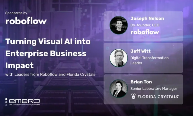
To address these systemic barriers, Emerj recently conducted a series of deep-dive discussions with industry leaders who have successfully navigated the transition from pilot to production. The series featured Joseph Nelson, co-founder and CEO of Roboflow; Jeff Witt, a manufacturing IT veteran managing vision programs across more than 100 facilities; and Brian Ton, Senior Laboratory Manager at Florida Crystals Corporation. Their collective insights reveal that scaling computer vision is less a technical hurdle and more a matter of ecosystem readiness, program ownership, and the strategic cultivation of operational trust.
The Foundation of Ecosystem Readiness
Joseph Nelson of Roboflow posits that the failure of most vision systems stems from a lack of "ecosystem readiness." In his view, a high-performing model is useless if the surrounding physical and digital infrastructure is not prepared to support it. This readiness is defined by three critical layers: data capture, model specificity, and downstream integration.
Data readiness begins with the physical placement of hardware. Many manufacturers attempt to deploy AI using existing security cameras that were never intended for quality control. Nelson emphasizes that organizations must first ask whether they have sensors positioned to capture the specific visual data required—such as the cross-section of a battery or the precise alignment of a stamping press. Without high-quality, task-specific visual data, the most advanced model has nothing of value to process.
Furthermore, Nelson argues against the reliance on purely general-purpose AI models for specialized manufacturing tasks. While foundation models are improving, the nuances of a specific assembly line—varying lighting conditions, unique product materials, and specialized defect types—require models trained on an organization’s proprietary data. The final piece of the puzzle is downstream integration. A system that identifies a missing screw provides zero business value if that information remains siloed within the vision software. The intelligence must be piped directly into Manufacturing Execution Systems (MES), quality management platforms, or the handheld devices of floor operators to trigger real-time corrective actions.
Nelson cites BNSF Railway as a prime example of successful scaling. By monitoring 30,000 miles of track and millions of containers through visual AI, the railroad has automated wheel inspections and track condition monitoring. However, the value is not in the detection alone; it is in the automated scheduling of maintenance crews and the real-time dispatching systems that respond to the AI’s findings. Nelson advocates for a "barbell strategy": maintaining a high-level executive vision for the future while focusing on a highly specific, bounded use case at the line level to prove immediate ROI.
Shifting Ownership from IT to Operations
A recurring theme in the history of industrial technology is the friction between Information Technology (IT) and Operational Technology (OT). Jeff Witt, a digital transformation leader with experience across a vast manufacturing network, argues that computer vision projects often stall when they are treated as IT-led software deployments rather than business-led operational upgrades.
Witt notes that many facilities are already "camera-rich," but those cameras are often locked within isolated IT networks, disconnected from the data pipelines that drive business intelligence. To scale, Witt’s team focused on breaking down these silos, ensuring that vision data could be combined with other process data (such as temperature, pressure, or vibration) to provide a holistic view of asset health.
Crucially, Witt found that adoption accelerated when the "keys to the kingdom" were handed to the plant managers and operators. When IT serves as a gatekeeper, the feedback loop between the model and the real-world application is too slow. By empowering business units to define their own use cases and manage their own models via accessible platforms, organizations can replicate success across similar production lines in multiple geographic locations.
Witt also challenges the "perfectionist" mindset that often delays AI deployment. In his experience, a model does not need to be 100 percent perfect to provide immediate value. Even a system that provides "meaningful operational visibility" or early anomaly detection can save a company millions in waste before it is fully optimized. The visual nature of the technology serves as its own change-management tool; when operators can see the AI highlighting a defect on a screen in real-time, the "black box" of AI becomes a transparent, trusted tool.
Building Operational Trust Through Small Victories
The human element remains perhaps the most significant barrier to AI adoption. Brian Ton of Florida Crystals Corporation observes that many projects fail because they do not account for the practical realities of the people working on the floor. If a system is designed in a vacuum by data scientists without input from the technicians and quality staff who understand the nuances of the production shift, it will inevitably miss critical edge cases.
Ton emphasizes that operational trust is not granted upon the installation of a system; it is earned through "small, manageable victories." In the complex environment of sugar refining and food production, introducing a massive, enterprise-wide AI overhaul is often a recipe for resistance. Instead, Ton suggests starting with a single, easy-to-understand problem—such as a specific measurement in a laboratory setting—and proving that the AI can handle it more consistently than a manual process.
Once the AI demonstrates it can increase data processing volumes by orders of magnitude without increasing the workload of the staff, the "credibility gap" closes. This allows the organization to transition from line-level implementations to site-level and, eventually, enterprise-level deployments. Ton’s experience suggests that the productivity upside of visual AI is a "multiplier of throughput," but reaching that upside requires a humble, incremental approach to deployment.
Chronology and Evolution of Vision AI in Industry
The journey of computer vision in manufacturing has evolved through several distinct phases:
- Traditional Machine Vision (1980s–2010s): Rule-based systems that used high-contrast lighting and rigid algorithms to detect simple shapes or barcodes. These were effective but brittle, requiring expensive re-programming for every minor product change.
- The Deep Learning Breakthrough (2012–2018): The rise of Convolutional Neural Networks (CNNs) allowed computers to "see" with human-like nuance. However, these models required massive computing power and specialized expertise.
- The Era of Pilot Purgatory (2018–Present): While the technology became accessible, the "integration gap" emerged. Companies realized that having a smart model was different from having a smart factory.
- The Future of Resilient Manufacturing: The current shift toward "Physical AI" and Edge Computing, where intelligence is deployed directly onto the factory floor, integrated with the workforce and existing machinery.
Implications and Future Outlook
The findings from these industry experts suggest a significant shift in how manufacturing leaders should approach AI investment. The "technical" problem of computer vision has largely been solved; the "organizational" problem is the new frontier. As global supply chains face increasing pressure to be more resilient and efficient, the companies that successfully scale computer vision will be those that treat it as a core operational capability rather than an experimental IT project.
Data from the NIST report suggests that the move toward "Resilient Manufacturing" will require standardized protocols for how AI interacts with legacy hardware. Without these standards, the cost of custom integration will continue to keep 77 percent of projects in the pilot phase. However, as platforms like Roboflow and others democratize the ability to train and deploy models, the barrier to entry is falling.
The long-term implication is a fundamental change in the manufacturing workforce. Instead of performing repetitive visual inspections, human workers will increasingly move into "human-in-the-loop" roles, supervising AI systems and handling the complex edge cases that the models flag. This shift promises not only higher quality and lower waste but also a more agile manufacturing sector capable of responding to market changes in real-time. For the modern enterprise, the message is clear: the path out of pilot purgatory is paved with integrated data, operational ownership, and the steady accumulation of trust on the factory floor.
Related posts: