The Indispensable Foundation of Algorithmic Trading: Mastering Financial Data Infrastructure

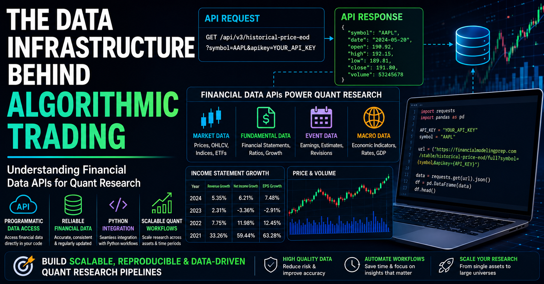
In the sophisticated world of algorithmic trading, the intricate dance of models, signals, and execution logic often overshadows a more fundamental, yet critically important, component: reliable access to financial data. Before any complex algorithms can be conceived or deployed, the bedrock of accurate and consistent data must be firmly established. In professional quantitative research environments, the data infrastructure is not merely a preliminary step; it is a decisive gating function. Any instability or inconsistency at this foundational layer inevitably propagates through every subsequent downstream model, compromising the integrity of the entire trading system. This exploration delves into the core of systematic trading’s data infrastructure, examining how financial data APIs, such as those provided by Financial Modeling Prep (FMP), facilitate automated data ingestion, integrate seamlessly into quantitative research pipelines, and empower developers to construct scalable research workflows using Python.

Why Data Infrastructure Reigns Supreme in Algorithmic Trading

The efficacy and reliability of any quantitative trading workflow, particularly when operating at scale, are directly dictated by its underlying data infrastructure. The ability to rigorously evaluate models or test trading signals hinges on the assurance that financial data is not only available but also presented in a structured, consistent, and scalable format. Without this robust foundation, even the most elegantly designed trading strategies can become exceedingly difficult to validate, reproduce, or trust in real-world applications.

The Imperative of Reliable Data Inputs for Systematic Trading

Challenges within data infrastructure are often insidious, rarely revealing themselves at the outset of a project. Minor inconsistencies in data inputs—such as intermittent missing values, misaligned timestamps across different data sources, or subtle formatting discrepancies—can compound as they traverse the data pipeline. This cascading effect can significantly distort feature calculations, skew model outputs, and ultimately render backtest results unreliable, leading to flawed strategic decisions.

Data Demands in Quantitative Research

Quantitative research workflows are inherently data-intensive, relying on the seamless integration of multiple disparate datasets. These typically include high-frequency price data, detailed financial statements, and event-driven information like corporate news or regulatory filings. As research initiatives expand in scope—encompassing larger universes of securities or delving into extended historical time periods—the complexity of managing these datasets escalates dramatically, underscoring the necessity of a well-architected data infrastructure.

The Inefficiencies of Manual Data Collection

In the absence of automated data retrieval mechanisms, the process of data collection quickly devolves into an inefficient and error-prone endeavor. Manual workflows, which often involve downloading individual spreadsheets, copying data from disparate online sources, or manually parsing reports, introduce a host of limitations. While these methods might suffice for rudimentary analyses or small-scale explorations, they are fundamentally incapable of scaling to meet the demands of professional quantitative research.

The common issues encountered with manual data collection are manifold:

• Time Consumption: Manually gathering and organizing data from various sources consumes a significant amount of researcher time that could otherwise be dedicated to analysis and strategy development.
• Error Proneness: Human error is an inherent risk in manual data entry and manipulation, leading to inaccuracies that can compromise the integrity of research findings.
• Lack of Standardization: Data from different sources often comes in varying formats, requiring extensive cleaning and standardization, which is time-consuming and introduces further opportunities for error.
• Difficulty in Updates: Keeping manual datasets up-to-date requires repetitive manual effort, making it challenging to implement timely re-runs of analyses or adapt to changing market conditions.
• Reproducibility Issues: The manual steps involved make it difficult for other researchers, or even the original researcher at a later date, to precisely replicate the data collection process and, consequently, the research outcomes.

These challenges collectively contribute to a pervasive lack of consistency, making it exceptionally difficult to validate research outcomes over time or to ensure the reproducibility of critical analytical results.

Financial Data APIs: The Cornerstone of Modern Infrastructure

Financial data APIs (Application Programming Interfaces) provide a structured and automated pathway to retrieve datasets directly into a research environment, effectively supplanting cumbersome manual workflows with programmatic access. Within quantitative research pipelines, these APIs primarily serve the critical function of the data ingestion layer. They enable the retrieval and direct integration of essential datasets—such as historical prices, comprehensive financial statements, and analyst estimates—directly into the analytical workflow. This programmatic approach fosters repeatable data access, simplifies integration with popular Python-based research environments, and ultimately facilitates more scalable and robust research processes.

Understanding Financial Data APIs

A financial data API acts as a programmatic interface, granting access to vast repositories of financial datasets. This allows data to be retrieved directly within code, eliminating the need for manual downloads and subsequent manipulation. Essentially, it functions as a bridge between a data provider and a research environment, enabling data to be requested and consumed programmatically. In practice, developers evaluate APIs not only on the breadth and depth of data provided but also on crucial technical specifications such as latency (the time delay in data retrieval), rate limits (the number of requests allowed within a given period), schema consistency (the predictability of data structure), and the overall reliability of API endpoints when handling large-scale requests.

For quantitative researchers working with Python, this translates into the ability for a script or notebook to effortlessly retrieve datasets—including historical price data, detailed financial statements, or forward-looking analyst estimates—without any reliance on manual data collection methods.

How an API Works in Practice

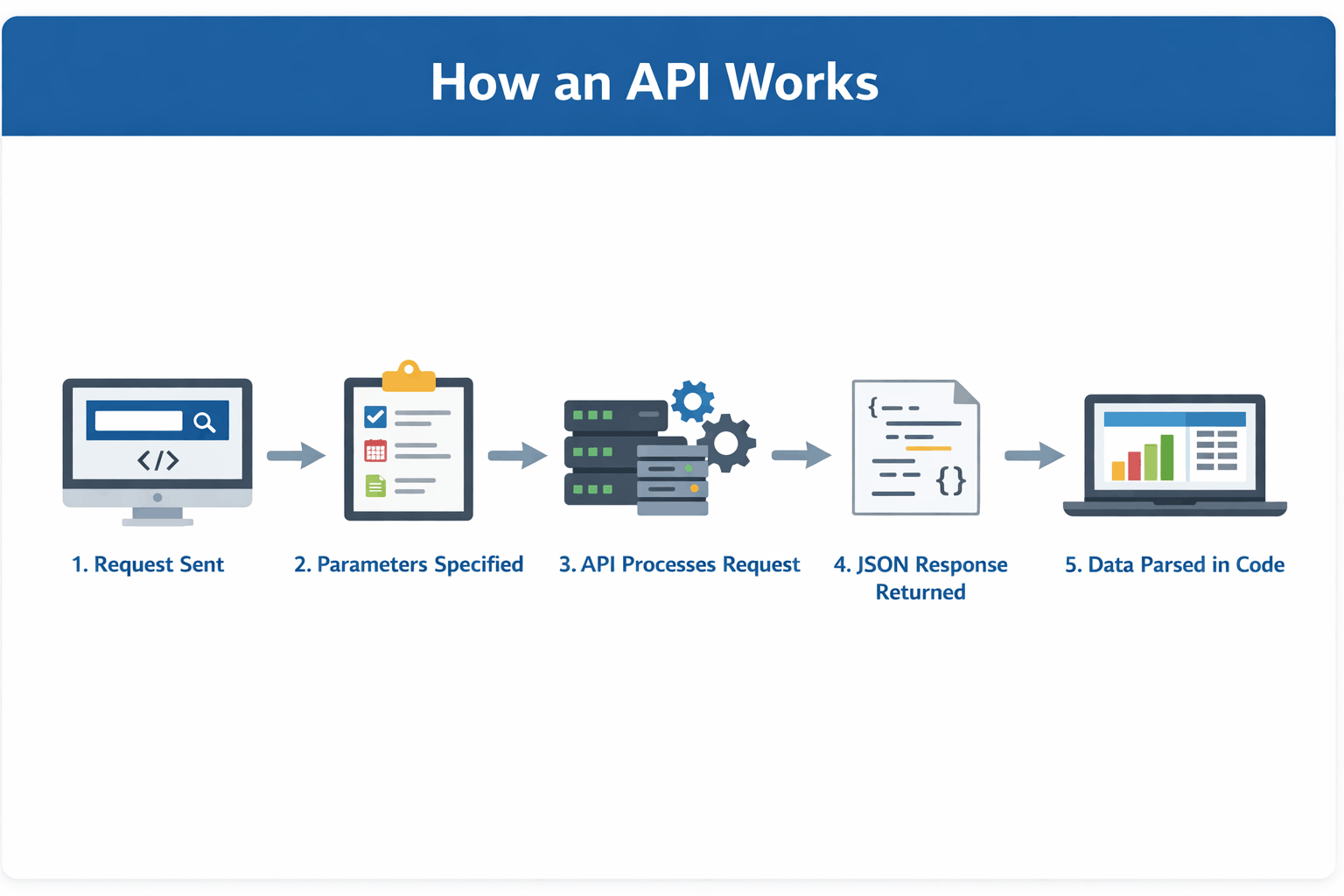
The interaction between a user and a financial data API typically follows a standard request-response model. A user’s application (e.g., a Python script) sends a request to a specific API endpoint, specifying the desired data (e.g., AAPL’s historical prices for the last year). The API server processes this request, retrieves the relevant data from its database, and returns it in a structured format (often JSON or CSV) to the user’s application. This structured output can then be directly parsed and used within the research environment.

For instance, financial data platforms commonly expose endpoints for a wide array of datasets. These might include company profiles, historical price data (open, high, low, close, volume), and detailed financial statements (income statements, balance sheets, cash flow statements). Each of these datasets is accessed and delivered through the consistent request-response pattern inherent to API functionality.

Manual Versus Programmatic Data Retrieval: A Comparative Analysis

The stark differences between manual data collection methods and API-driven programmatic retrieval become readily apparent when examining key operational aspects:

Aspect	Manual Data Retrieval	Programmatic Data Retrieval
Effort	High (repeated manual steps, prone to fatigue)	Low (automated through code, once set up)
Scalability	Limited to small datasets and infrequent updates	Scales efficiently across large datasets and volumes
Consistency	Prone to formatting inconsistencies and human error	Standardized, structured, and inherently consistent
Update Process	Requires continuous manual intervention	Automatically refreshable with scheduled scripts
Reproducibility	Difficult to replicate precisely	Fully reproducible workflows with version-controlled code

For quantitative research, the benefits of programmatic access are profound. It significantly reduces human intervention, thereby minimizing errors and ensuring a higher degree of data consistency. This reliability is paramount for building trustworthy analytical models and trading strategies.

Authentication: Securing Access with API Keys

Most financial data APIs employ an authentication mechanism, typically through the use of API keys. This unique key is included with each request made to the API. Its primary purpose is to verify the user’s identity, enabling the data provider to manage access permissions and enforce usage limits. This ensures that only authorized users can access the data and that usage stays within agreed-upon parameters.

The Centrality of APIs in Quantitative Workflows

Financial data APIs fundamentally transform data access from a manual, often tedious, preparatory task into a programmable, integrated component of the research pipeline. Instead of dedicating significant time to data preparation, researchers can now embed data retrieval directly into their code. This seamless integration leads to consistently reliable data inputs, accelerates the iterative process of model development and testing, and fosters the creation of truly scalable research workflows. Consequently, APIs have become an indispensable element of modern quantitative research environments, underpinning the efficiency and robustness of systematic trading operations.

Key Financial Data Types for Algorithmic Trading

Once programmatic access to financial data is established, the next critical step involves understanding the diverse types of datasets commonly employed in quantitative research. These datasets serve as the foundational input layer for most research pipelines and are typically retrieved via financial data APIs.

Type of Data	Examples
Market Data	Historical price data (open, high, low, close, volume), intraday price series, index and ETF prices
Fundamental Data	Income statements (revenue, net income), balance sheets (assets, liabilities), cash flow statements, financial ratios
Event & Macro Data	Earnings calendars, analyst estimates and revisions, economic indicators (inflation, interest rates, GDP)

These datasets collectively form the essential input layer for a vast array of quantitative research workflows, all of which are typically accessed through sophisticated financial data APIs.

To illustrate how financial data APIs practically support real-world workflows, let us consider a simplified research scenario. The objective here is not to construct a fully functional trading strategy, but rather to demonstrate the flow of data through a structured pipeline, emphasizing the use of reliable and repeatable data sources.

A Practical Research Scenario: Fundamentals and Price Behavior

Imagine a researcher aiming to determine whether improvements in a company’s fundamental financial health can serve as a consistent cross-sectional signal across a broad universe of equities. This research objective necessitates the integration of multiple datasets, specifically analyzing how trends in financial performance correlate with observed price movements across different companies. Such workflows are commonly taught in structured quantitative finance programs and closely mirror the methodologies employed in both academic and professional quant environments.

Essential APIs for This Workflow

Before constructing the analytical pipeline, it is crucial to define the required datasets and the APIs needed to access them. For this scenario, two primary data types are essential:

1. Historical Price Data: This dataset is required to retrieve end-of-day price data, which will be used for time-series analysis of stock price behavior.
2. Income Statement Growth Data: This dataset will provide access to key growth metrics, such as revenue growth and earnings growth, enabling an assessment of fundamental financial trajectory.

Acquiring Your API Key: The Gateway to Data

To access most financial data APIs, users typically need to register for an API key. This key is then incorporated into subsequent API requests for authentication and usage tracking purposes. For instance, registering at Financial Modeling Prep (FMP) provides access to their extensive financial data. Following registration, the API key is made available in the user’s dashboard. This key will need to be substituted for placeholder values (e.g., "YOUR_API_KEY") in any code examples used to authenticate requests.

Step 1: Data Ingestion – The Foundation of the Pipeline

The initial phase of the research pipeline involves retrieving structured datasets using financial data APIs. Rather than resorting to manual data collection, the process focuses on fetching both market data and fundamental data programmatically.

Fetching Historical Price Data

The process begins with retrieving end-of-day price data, which will serve as the basis for analyzing price movements over time.

import requests
import pandas as pd

API_KEY = "YOUR_API_KEY"  # Replace with your actual API key
symbol = "AAPL"  # Example: Apple Inc.
url = f"https://financialmodelingprep.com/stable/historical-price-eod/full?symbol=symbol&apikey=API_KEY"
response = requests.get(url)
data = response.json()
prices = pd.DataFrame(data)
prices.head()

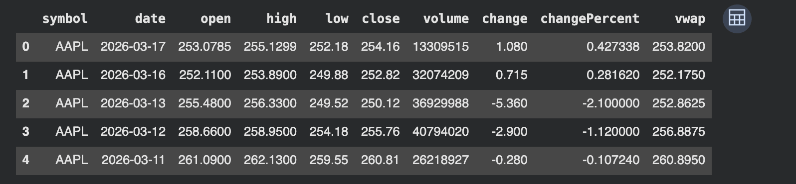
The output from this code snippet will typically display structured end-of-day price data for the specified symbol (e.g., Apple) in a clean, tabular format. Each row represents a trading day, and the columns detail key market metrics such as open price, high price, low price, closing price, trading volume, daily price change, percentage change, and Volume Weighted Average Price (VWAP).

This structured output is invaluable because the dataset is immediately usable within a research environment without requiring extensive manual formatting. Researchers can readily sort the data by date, filter for specific time periods, compute rolling statistical measures, align price movements with fundamental events, or merge this table with other relevant datasets, such as income statement growth figures or analyst consensus estimates.

Fetching Fundamental Growth Data

To effectively support the research objective, it is also necessary to retrieve fundamental growth metrics. These datasets are crucial for capturing the trajectory of a company’s financial performance over time.

growth_url = f"https://financialmodelingprep.com/stable/income-statement-growth?symbol=symbol&apikey=API_KEY"
growth_response = requests.get(growth_url)
growth_data = growth_response.json()
growth_df = pd.DataFrame(growth_data)
growth_df.head()

Interpretation of Fundamental Growth Data

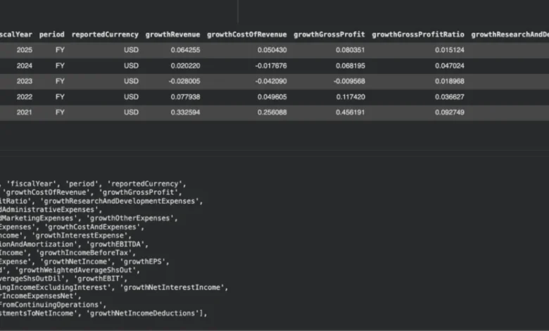
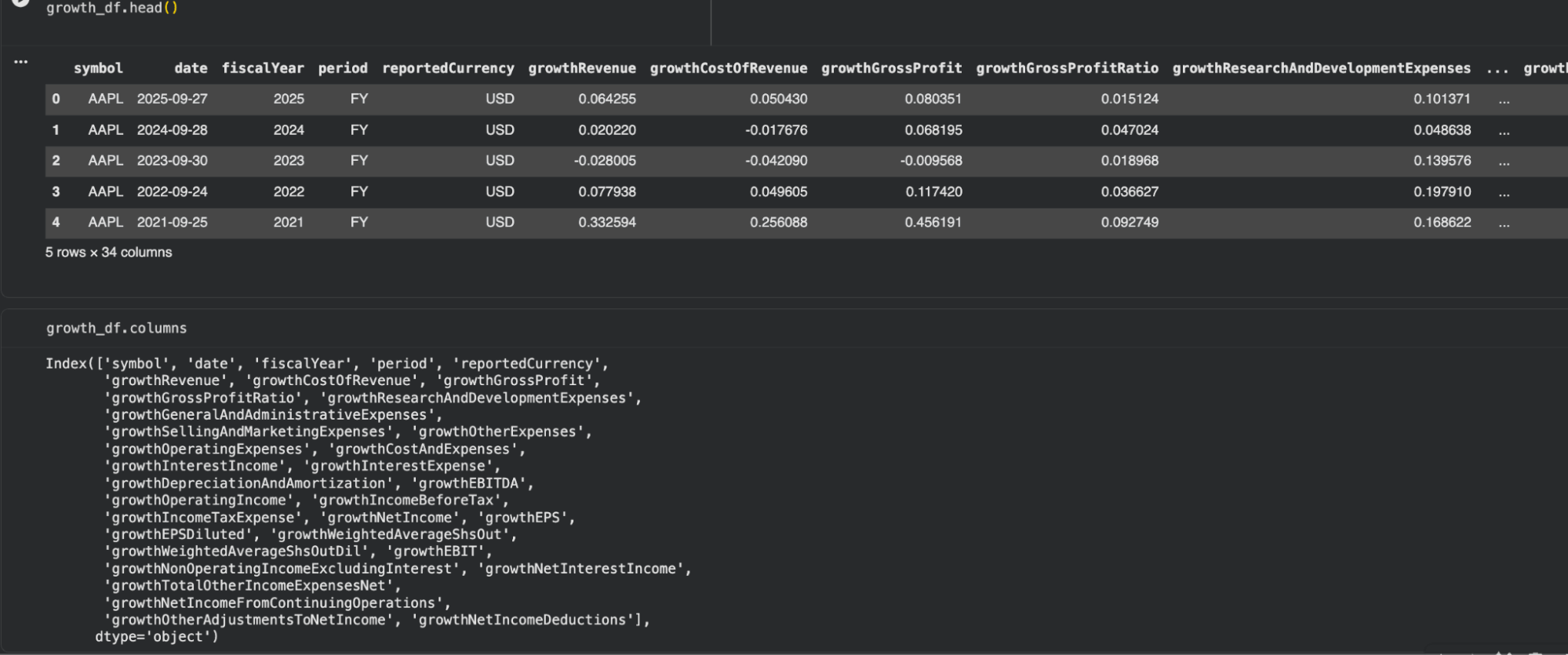
The output from this request reveals structured fundamental growth data for the company across multiple fiscal years. Each row typically corresponds to a distinct reporting period, while the columns encapsulate growth metrics derived from various components of the income statement.

Key observations from such a dataset commonly include:

• Year-over-Year Growth Rates: Explicit calculations of percentage growth for revenue, net income, and earnings per share (EPS) on an annual basis.
• Segment-Specific Growth: In some cases, growth rates for specific business segments or product lines might be available, providing deeper insights.
• Consistency and Standardization: The data is usually preprocessed, meaning growth values are directly available without the need for manual calculation. This significantly reduces preprocessing effort and ensures consistency across different companies analyzed.

A critical aspect of this dataset is its time granularity. Unlike price data, which is often available on a daily basis, fundamental data is reported at a financial period level (typically annually or quarterly). This difference in frequency becomes a significant consideration when integrating datasets later in the pipeline. Overall, this dataset provides a clear picture of how a company’s fundamentals are evolving, complementing the price-based dataset that was retrieved earlier.

Step 2: Feature Engineering – Transforming Raw Data into Insights

With both market data and fundamental data successfully ingested, the subsequent step involves transforming these raw datasets into structured variables that can effectively support quantitative analysis.

Engineering Price-Based Features

The initial stage of feature engineering focuses on deriving meaningful features from the historical price dataset.

# Convert date column to datetime objects for proper sorting
prices['date'] = pd.to_datetime(prices['date'])
prices = prices.sort_values("date").reset_index(drop=True)

prices["daily_return"] = prices["close"].pct_change()
prices["price_range"] = prices["high"] - prices["low"]
prices["rolling_5d_avg_close"] = prices["close"].rolling(5).mean()
prices["rolling_5d_volatility"] = prices["daily_return"].rolling(5).std()

# Displaying a subset of engineered features
print(prices[["date", "close", "daily_return", "price_range", "rolling_5d_avg_close", "rolling_5d_volatility"]].head(10))

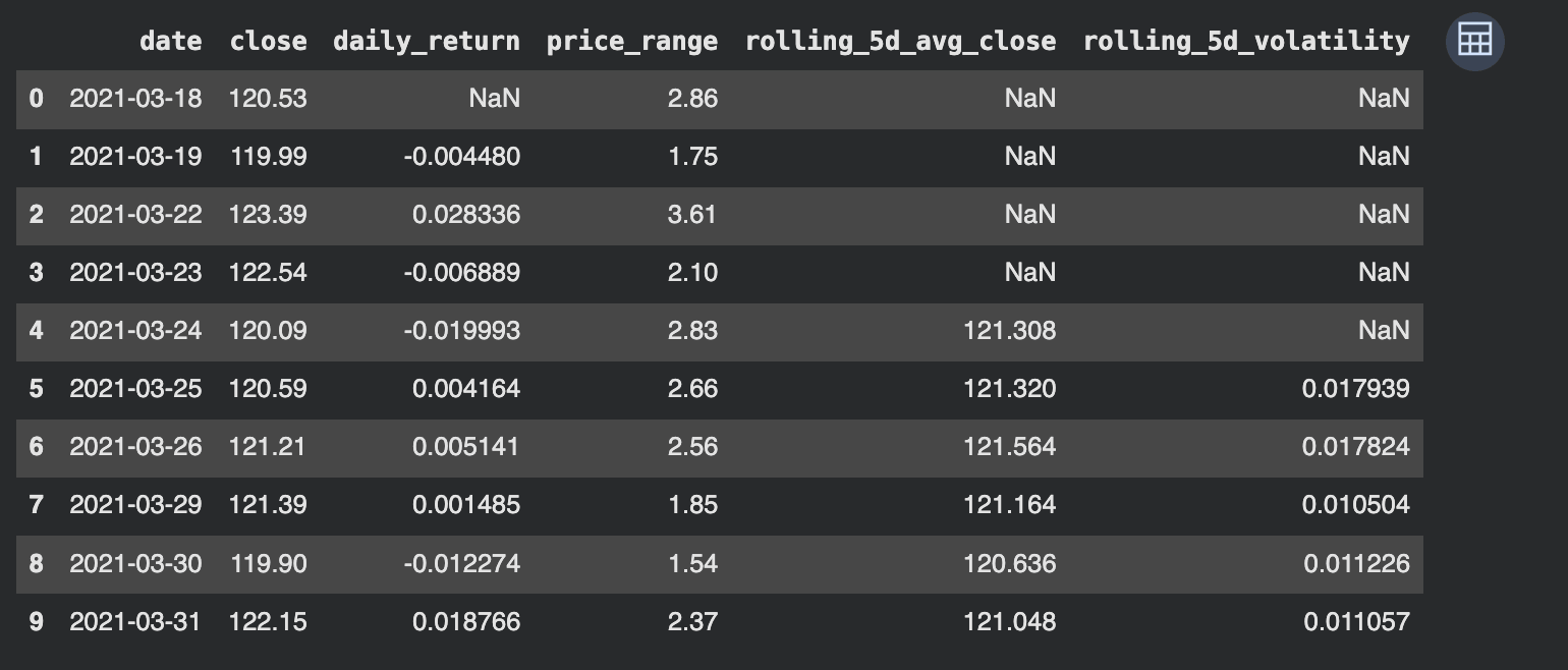
The resulting engineered dataset demonstrates how raw price data has been transformed into structured features suitable for analytical purposes. Each newly created feature captures a distinct aspect of market behavior:

• Daily Return: Measures the percentage change in the closing price from one trading day to the next, a fundamental metric for assessing short-term price movement.
• Price Range: Represents the difference between the high and low price for a given trading day, indicating intra-day price volatility.
• Rolling 5-Day Average Close: Calculates the average closing price over a rolling 5-day window, smoothing out short-term fluctuations and identifying underlying trends.
• Rolling 5-Day Volatility: Computes the standard deviation of daily returns over a rolling 5-day period, quantifying short-term price volatility.

Initial occurrences of NaN (Not a Number) values are expected in these rolling calculations, as they require a minimum number of preceding observations to be computed. This step is crucial as it converts raw market data into features that can be consistently compared across different time periods and readily integrated with other datasets, such as financial statements or analyst estimates.

Working with Fundamental Growth Features

In contrast to market data, the fundamental dataset often provides pre-engineered growth variables directly. These can typically be utilized without requiring further transformation. Examples of these readily available features include:

• Revenue Growth: The year-over-year percentage increase in total revenue.
• Net Income Growth: The year-over-year percentage increase in net income.
• EPS Growth: The year-over-year percentage increase in earnings per share.

These variables effectively describe the evolving financial performance of a company, a critical element in many research workflows.

Aligning Price and Fundamental Data: A Critical Integration Step

A particularly important aspect of feature engineering is the alignment of datasets that operate at different frequencies. Misalignment between reporting periods for fundamental data and corresponding price data is a pervasive source of bias in quantitative research, especially when fundamental data is improperly forward-filled.

To effectively combine these datasets, researchers typically map fundamental values to the relevant price periods. This can be achieved through various techniques, including:

• Date-Based Mapping: Directly matching fundamental reporting dates with corresponding price data.
• Forward Filling: Assigning the fundamental value from the most recent reporting period to all subsequent daily price observations until a new fundamental report is released.
• Backward Filling: Less common, but potentially used in specific scenarios to fill missing fundamental data points based on prior reports.

The following simplified example illustrates how these datasets can be aligned programmatically:

# Convert date columns to datetime objects for accurate merging and sorting
prices["date"] = pd.to_datetime(prices["date"])
growth_df["date"] = pd.to_datetime(growth_df["date"])

# Merge datasets based on 'symbol' and 'date' columns using a left join
# This ensures all price data is retained, and matching fundamental data is added.
merged_df = prices.merge(growth_df, on=["symbol", "date"], how="left")

# Sort the merged dataframe by date to ensure correct forward filling
merged_df = merged_df.sort_values("date")

# Forward fill the fundamental values across daily price data.
# This assigns the last known fundamental value to subsequent days until a new one is available.
merged_df = merged_df.ffill()

# Display the head of the merged dataframe to show the integrated data
print(merged_df.head())

This alignment process ensures that both market behavior and business performance metrics can be analyzed in tandem within a unified, coherent dataset.

Key Outcome of Feature Engineering

Upon completion of the feature engineering stage, the dataset is enriched and contains:

• Engineered Price-Based Features: Metrics derived from historical price data, such as daily returns, volatility, and moving averages, offering insights into market dynamics.
• Fundamental Growth Metrics: Direct indicators of a company’s financial performance evolution, like revenue and earnings growth rates.
• Aligned Data: Market and fundamental data are synchronized, enabling direct comparison and analysis of their interrelationships.

This integrated dataset empowers more meaningful analysis, allowing researchers to evaluate price behavior in the context of a company’s underlying financial health and performance trends.

Step 3: Hypothesis Testing – Uncovering Relationships

With both price-based features and fundamental growth data now readily available and aligned, the researcher can commence the structured evaluation of relationships within the data. The objective at this stage is not to develop a fully operational trading strategy, but rather to rigorously test whether observable patterns exist between market behavior and a company’s underlying business performance.

Defining the Research Question

A concise and relevant hypothesis for this scenario could be: "Do periods of stable price behavior systematically align with periods of improving company fundamentals?" This question seeks to connect two critical dimensions:

• Market Dynamics: Characterized by price stability, indicating low volatility or predictable price movements.
• Business Performance: Reflected in the trajectory of fundamental metrics, such as increasing revenue and profitability.

Structuring the Analysis

To evaluate this hypothesis, the researcher can undertake the following analytical steps:

1. Identify Periods of Stable Price Behavior: Define criteria to identify time intervals characterized by low price volatility (e.g., using rolling volatility metrics).
2. Analyze Fundamental Trends During Stable Periods: Examine the behavior of fundamental growth metrics (e.g., revenue growth, EPS growth) during these identified periods of price stability.
3. Compare with Volatile Periods: Contrast the fundamental trends observed during stable periods with those during periods of higher price volatility to identify significant differences.
4. Quantify the Relationship: Employ statistical methods to measure the strength and significance of any observed correlation between price stability and fundamental improvement.

Example Workflow: Identifying Low Volatility Periods

A simplified analytical approach could involve filtering the data to isolate periods of low volatility:

# Example: Identify periods of low volatility using the 30th percentile of rolling 5-day volatility
low_volatility_threshold = prices["rolling_5d_volatility"].quantile(0.3)
low_volatility_periods = prices[prices["rolling_5d_volatility"] < low_volatility_threshold]

# Displaying a subset of the data filtered for low volatility periods
print(low_volatility_periods[["date", "close", "rolling_5d_volatility"]].head())

The filtered dataset visually highlights periods where short-term price volatility was relatively low, based on the lower quantile of the rolling 5-day volatility.

From such a sample, observations might include:

• Specific Dates: Identification of trading days falling within periods of low volatility.
• Associated Prices: The closing prices on those specific dates.
• Volatility Levels: The measured rolling 5-day volatility values, confirming they are below the established threshold.

This output demonstrates that:

• Periods of Calm Identified: The filtering process successfully isolates periods of relative calm in the market.
• Data Integrity Maintained: The associated price and volatility data remain consistent and reliable.

This process exemplifies how combining price-based features with fundamental growth data enables a more structured evaluation of market behavior. It facilitates a transition from merely observing descriptive patterns to conducting testable, data-driven relationships.

Step 4: Scaling the Research – From Single Stock to Universe

In most professional quantitative research environments, research pipelines are architected from the outset to operate across hundreds or even thousands of securities. This makes scalability not merely an optimization goal but a core design requirement.

Once a research workflow has been thoroughly validated for a single company, the same pipeline can be efficiently extended to encompass a larger universe of securities. Because both the data ingestion and feature engineering processes are implemented in code, the entire process can be replicated with minimal modifications.

In practice, scaling such a research pipeline may involve several considerations:

• Batch Processing: Implementing loops or batch processing mechanisms to execute the data retrieval and analysis for each security in the universe.
• Parallelization: Utilizing parallel processing techniques to distribute the computational load across multiple processor cores or machines, significantly accelerating execution times.
• Database Integration: Storing processed data and features in a robust database for efficient querying and further analysis.
• Cloud Infrastructure: Leveraging cloud computing platforms for scalable storage, processing power, and orchestration of research workflows.

For example, the identical feature engineering logic applied to Apple’s data can be readily applied to hundreds of other stocks by simply iterating through a list of symbols. This is where financial data APIs play an indispensable role. They empower researchers to transition from isolated, single-stock examples to robust, scalable research systems, where data retrieval, transformation, and analysis can be executed with consistency and efficiency across vast datasets.

The Paramount Importance of Data Quality in Systematic Trading

As the research pipeline becomes more structured and repeatable, the ultimate reliability of any analysis is still fundamentally contingent upon the quality of the underlying data. Even the most sophisticated workflows can yield misleading results if the input data is incomplete, inconsistent, or improperly adjusted. Data quality is not merely a technical concern; it has a direct and profound impact on the accuracy with which researchers can evaluate patterns, compare disparate entities, and validate hypotheses.

Common Data Issues in Quantitative Research

Financial datasets frequently contain subtle issues that, while not immediately apparent, can significantly compromise analytical outcomes. These common challenges include:

• Survivorship Bias: Occurs when historical data only includes entities that have survived to the present, leading to an overestimation of past performance.
• Lookahead Bias: Arises from inadvertently using future information in historical analysis, often due to incorrect timestamping or data merging.
• Missing Historical Records: Gaps in historical data can lead to incomplete analyses and biased conclusions.
• Improper Handling of Corporate Actions: Failure to accurately adjust for events like stock splits, dividends, or mergers can distort historical price and fundamental data.

These issues become particularly pronounced and problematic when scaling analysis across numerous securities or extended historical time periods.

Impact on Research Outcomes

Data quality directly influences every stage of the research pipeline, from the initial feature engineering to the final hypothesis testing. Inconsistent, incomplete, or erroneous data can lead to:

• Distorted Signals: Trading signals derived from flawed data will be unreliable and potentially lead to adverse trading decisions.
• Unreliable Comparisons: Comparing companies or time periods based on inaccurate data will yield misleading insights.
• Misleading Conclusions: The ultimate findings and strategic recommendations derived from the research can be fundamentally flawed.

The Role of Financial Data APIs in Enhancing Data Quality

Reliable financial data APIs significantly mitigate many of these data quality challenges by providing standardized and structured datasets. With consistent schemas, preprocessed metrics, and regular updates, APIs simplify the process of integrating multiple datasets into a unified and coherent research pipeline. This standardization reduces the burden of manual data cleaning and validation, allowing researchers to focus on higher-value analytical tasks.

Why Data Quality Is the Foundational Layer

Data quality directly underpins the credibility and trustworthiness of quantitative research. When the input data is reliable:

• Research Reproducibility is Ensured: Other researchers can confidently replicate findings.
• Model Performance is Accurately Assessed: The true efficacy of models can be determined.
• Decision-Making is Informed: Strategic decisions are based on sound, data-driven insights.
• Risk is Effectively Managed: A clear understanding of data limitations allows for better risk assessment.

Conversely, if the input data is flawed:

• Models Produce Erroneous Signals: Leading to poor trading performance.
• Backtests Become Unreliable: Historical simulations do not reflect real-world outcomes.
• Investment Strategies Are Compromised: Decisions are based on flawed premises.

This underscores why data quality is considered the foundational layer in systematic trading. Before any hypothesis can be rigorously evaluated, researchers must ensure that the data underpinning their analysis is accurate, consistent, and complete.

Key Takeaways

• Data Infrastructure is Paramount: The reliability and scalability of financial data access form the bedrock of successful algorithmic trading and quantitative research.
• APIs Streamline Processes: Financial data APIs automate data ingestion, integrate seamlessly into research pipelines, and enable scalable workflows.
• Data Quality is Non-Negotiable: Inconsistent or incomplete data can lead to flawed analysis, unreliable signals, and ultimately, poor trading performance.
• Structured Approach is Essential: A systematic approach to data ingestion, feature engineering, and hypothesis testing, facilitated by robust data infrastructure, is crucial for credible research.

About the Contributor

Financial Modeling Prep (FMP) is a leading provider of structured financial data APIs, serving the needs of quantitative researchers, investment analysts, and developers. Its platform is engineered to facilitate scalable and efficient access to a comprehensive suite of datasets, including market data, financial statements, analyst estimates, and other critical information essential for systematic research environments.

---

Disclaimer: All data and information provided in this article are for informational purposes only. QuantInsti® makes no representations as to accuracy, completeness, currentness, suitability, or validity of any information in this article and will not be liable for any errors, omissions, or delays in this information or any losses, injuries, or damages arising from its display or use. All information is provided on an as-is basis.