LLM-Powered Trading Strategy Reimagined: Shifting Focus from Prediction to Risk Management

Many ambitious attempts to leverage Large Language Models (LLMs) in trading strategies have faltered, largely due to an inherent difficulty in reliably predicting future market returns. As noted by E.P. Chan in 2024, this fundamental challenge renders traditional predictive models, regardless of their sophistication, unreliable for anticipating tomorrow’s market movements. Building on this crucial insight, a novel strategy has emerged, tasking an LLM not with forecasting market direction, but with acting as a sophisticated risk manager. This approach centers on the LLM’s ability to dynamically adjust investment allocations based on perceived market risk, rather than attempting to divine future price movements.

The core innovation of this strategy lies in its redefinition of the LLM’s role. Instead of posing the question, "Will the stock go up or down tomorrow?" – a notoriously difficult prediction task for even the most advanced AI – the LLM is prompted with a more manageable and potentially more impactful query: "Given the historical behavior of this stock across different market states over the past three years, does the current state suggest a need for full investment, or should exposure be reduced?" This paradigm shift leverages the LLM’s capacity for nuanced interpretation of complex data patterns to inform risk assessment, a task where it can potentially offer a distinct advantage.

Strategic Framework: A Layered Approach to Risk Mitigation

This sophisticated trading system is meticulously constructed with a multi-layered architecture, designed to harness the analytical power of LLMs while incorporating robust safeguards against catastrophic losses. At its heart, a monthly walk-forward loop iteratively refines the LLM’s decision-making policy. This process ensures that the model’s directives remain adaptive to evolving market conditions. Concurrently, guardrail thresholds, the critical safety nets of the system, are also re-optimized on a monthly basis, aligning risk parameters with the LLM’s updated assessments.

The strategy employs a series of "hard guardrails" that operate independently of the LLM’s direct instructions. These include volatility stops, which trigger a reduction in exposure during periods of extreme price fluctuation, and drawdown stops, designed to halt further losses when the strategy’s equity falls below a predetermined threshold. A forced re-entry mechanism is also integrated to prevent the strategy from remaining sidelined indefinitely after a protective exit. Crucially, all performance evaluations and strategy validation are conducted rigorously out-of-sample (OOS) from January 2023 onwards, providing a realistic assessment of its efficacy in live market conditions.

Foundational Knowledge: Prerequisites for Understanding the Strategy

To fully grasp the intricacies of this LLM-driven trading strategy, a solid foundation in several key areas is beneficial. From a programming perspective, proficiency in Python, particularly with libraries such as pandas for data manipulation and numpy for numerical operations, is essential. Familiarity with making API calls using the requests library is also assumed. For those seeking to refresh these skills, comprehensive guides on Python for trading are readily available.

Beyond technical programming skills, a deep understanding of backtesting methodologies is paramount. This includes a clear grasp of out-of-sample evaluation, a critical technique for assessing a strategy’s predictive power on unseen data, and the computation of key performance metrics such as the Sharpe Ratio, Sortino Ratio, Calmar Ratio, and Maximum Drawdown. Educational resources dedicated to backtesting provide essential primers on these concepts.

On the strategic front, this approach sits at the intersection of three critical domains: market regime identification, LLM-assisted decision-making, and risk-aware position sizing. Understanding how to discretize continuous price signals into distinct market states, often achieved through techniques like Hidden Markov Models, provides conceptual grounding. The walk-forward loop, a cornerstone of robust strategy development, requires an understanding of its principles for more reliable backtesting. Furthermore, familiarity with position sizing techniques, particularly volatility targeting and the theoretical underpinnings of the Kelly criterion, is crucial for comprehending how capital is allocated.

The Introduction: Redefining the LLM’s Role in Trading

The primary reason many LLM-powered trading strategies have fallen short of expectations is the fundamental misapplication of their capabilities. Asking an LLM to predict daily price movements for highly liquid large-cap stocks, such as Apple (AAPL), is akin to asking it to predict the lottery numbers – a task for which no model, statistical, machine-learned, or language-based, possesses a reliable edge.

The breakthrough lies in reframing the LLM’s objective. Research has underscored the distinction between predicting returns and predicting volatility. Instead of forecasting direction, this strategy prompts the LLM to assess risk. The critical reframe is: "Given what I know about how this stock has behaved in each market state over the past three years, does today’s state look like one where I should be fully invested, or should I pull back?"

This strategy empowers DeepSeek, a powerful LLM, to analyze a table of historical statistics—including mean return, standard deviation, and a Sharpe-like score for each identified market state. Based on this analysis, the LLM outputs a policy dictating the appropriate investment allocation for each state. Notably, the strategy operates on a long-only basis, with investment ranging from 50% to 100% of capital. This calibrated, regime-aware exposure avoids the complexities and risks associated with shorting or leverage.

To ensure robustness, hard guardrails are implemented as a critical safety net. If realized volatility surges, confirmed by acceleration indicators, or if the strategy’s equity drawdown exceeds a predefined threshold, also with trend-break confirmation, the system automatically de-risks. A built-in re-entry mechanism prevents the strategy from remaining permanently inactive following a protective exit. By the conclusion of this detailed analysis, readers will possess a comprehensive understanding of every component of the implementation, from feature engineering and LLM prompting to the walk-forward backtesting loop.

Step 1: The Control Panel – Orchestrating the Experiment

Every rigorous backtest begins with a centralized "control panel"—a single configuration cell that governs the entire experimental setup. This panel defines three critical layers of settings: data parameters, cost assumptions, and the crucial exposure mapping that translates the LLM’s qualitative output into concrete position sizes.

The strategy defines three key exposure constants: LONG_FULL_EXP (representing 100% allocation), LONG_HALF_EXP (representing 50% allocation), and FLAT_EXP (also representing 50% allocation). These constants serve as the vital bridge between the LLM’s risk assessment and the portfolio’s actual risk exposure. The deliberate choice of FLAT_EXP at 0.5, rather than 0.0, is a strategic decision. It signifies that a cautious signal from the LLM translates to a reduction in exposure, not a complete exit from the market. This floor preserves the strategy’s participation in the market’s positive drift, even during periods of uncertainty.

Rationale for FLAT = 0.5: In a sustained bull market, such as the period observed for AAPL between 2023 and 2026, exiting the market entirely on every cautious signal could have resulted in a substantial loss of potential gains, estimated to be around 10 percentage points of Compound Annual Growth Rate (CAGR). Maintaining a 0.5 floor ensures continued market participation while still communicating the LLM’s risk-off sentiment.

Furthermore, settings such as MAX_FLAT_DAYS and REENTRY_SIZE are incorporated to address a subtle yet potentially devastating flaw known as the "guardrail deadlock." This issue, which can silently cripple a strategy’s performance, will be thoroughly examined in Step 5 when the guardrail logic is detailed.

Step 2: Data Integrity – The Foundation of Reliable Analysis

In the realm of algorithmic trading, the adage "garbage in, garbage out" holds particularly true. The acquisition of data is not merely about downloading historical prices; it is about acquiring the correct data. For a stock like AAPL, which has undergone multiple stock splits since 1990, this distinction is of paramount importance.

The auto_adjust=True flag is non-negotiable. Without this setting, historical data points corresponding to stock splits would generate artificially massive return spikes, contaminating all subsequent calculations. This includes rolling volatility, z-scores, trend scores, and virtually every other downstream metric. To mitigate this risk, a rigorous sanity check is implemented immediately after feature engineering:

# Example of a sanity check (conceptual)
if (data['Close'].pct_change().abs().rolling(20).mean().iloc[-1] > 0.1):
    raise ValueError("High recent volatility detected, check data adjustments.")

This type of defensive check, often requiring just a few lines of code, has proven instrumental in preventing backtests from yielding entirely erroneous results.

Step 3: Feature Engineering – Illuminating the Market’s Mood

Raw price data indicates the market’s position, but features illuminate its "mood." This strategy computes seven distinct signals derived from Open, High, Low, Close, and Volume (OHLCV) data. The overarching objective of this feature engineering process is to distill the current market state into a compact and interpretable set of indicators.

Traders and developers are encouraged to explore a broader array of features and technical indicators, leveraging libraries such as ta-lib, which offers a comprehensive suite of financial technical analysis functions. Installation guides for ta-lib in Python are readily available.

Step 4: Discretizing into Market States – Simplifying Complexity

Continuous features, while precise, can be challenging to reason about and can generate an overwhelming number of combinations. To address this, each signal is categorized into two or three distinct bins. These binned signals are then combined to form a single, composite "state string." The outcome is a manageable set of 12 distinct states, small enough for the LLM to effectively process and for each state to have a substantial number of historical examples for robust analysis.

Several design choices merit specific attention. The volatility threshold utilizes a rolling 252-day median rather than a fixed numerical value. This adaptive approach ensures that the volatility measure remains relevant across different market eras. What might have been considered "high volatility" in the low-volatility environment of 2017 would be considered "normal" in the post-COVID era. The rolling median automatically accounts for these shifts.

The resulting state strings are intentionally designed to be human-readable. When these descriptive states are presented to DeepSeek, the LLM can leverage its vast world knowledge to infer the historical implications of conditions like "trending upward in a calm, overbought market" for risk assessment. This qualitative judgment is precisely the type of insight sought from the model.

Step 5: The LLM Risk Manager – Constructing the Policy Table

This step represents the strategic core of the system. Once a month, DeepSeek is tasked with analyzing historical statistics for each market state and generating a policy table. This table dictates the recommended investment allocation for each state: whether to be fully invested, partially invested, or to pull back from the market.

The critical design decision here is how the task is framed for the LLM. While one might consider a strategy where the LLM predicts direction (LONG/SHORT/FLAT), this approach is inherently flawed. The optimal framing positions the LLM as a risk manager, not a forecaster.

Computing State Statistics: The process begins with calculating the statistics that the LLM will analyze. A one-day lag is incorporated into this function to prevent lookahead bias. Specifically, the market state observed at the close of day t-1 is used to inform the prediction for day t.

The sharpe_like column is arguably the most significant metric within this table. A strongly positive value indicates that, historically, when the market was in a particular state, AAPL exhibited favorable risk-reward characteristics on the subsequent day. Conversely, a strongly negative value suggests the opposite, while a value near zero implies inconclusive evidence.

The Prompt: Framing the LLM as a Risk Manager: The system prompt is the repository of the strategy’s underlying philosophy. Each sentence is deliberately chosen to guide the LLM’s decision-making process. Three guiding principles underpin this prompt design:

1. Explicit Task Reframing: The prompt explicitly states what the model should not do: "Your job is NOT to predict tomorrow’s price direction." This is followed by clear instructions on its actual role. LLMs are highly sensitive to task framing, and without this explicit redirection, they can revert to their default mode of direction forecasting.

2. Default to Action, Penalize Inaction: The prompt includes a "Default bias: LONG. Most states should be LONG." This directive counteracts the model’s natural inclination towards conservatism when faced with uncertainty. In a long-only strategy operating on a stock with a positive long-term drift, maintaining a "flat" position incurs a real opportunity cost – the missed positive expected return of the market.

3. Strict JSON Output with Retry: Requiring strict JSON output and providing the exact schema prevents the model from generating extraneous prose that could disrupt parsing. A retry mechanism and an increased max_tokens limit (to 2000) are also implemented. Earlier versions, with a lower token limit, occasionally truncated responses mid-JSON, leading to silent parsing failures.

Pro Tip: It is highly advisable to cache LLM responses. The cache_key should incorporate essential identifiers such as the month, symbol, model name, and a version tag (e.g., ‘longonly-v1’). This caching mechanism ensures that re-running backtests incurs minimal additional API calls once the cache is populated. The cache itself is a simple JSON dictionary, allowing for direct inspection of the LLM’s monthly decisions.

Step 6: From Policy to Position – Sizing with Volatility Targeting

The LLM’s output is a qualitative judgment—LONG full, LONG half, or FLAT. This needs to be translated into a precise numerical value: the fraction of capital to be invested. This conversion occurs in two stages: first, mapping the LLM’s action to a base exposure, and second, scaling this base exposure through volatility targeting.

Exposure Mapping: This mapping defines the strategy’s inherent risk-taking personality. The three defined exposure levels (1.0, 0.8, and 0.5) dictate how aggressively the LLM’s risk signals translate into actual position adjustments. These are tunable parameters within the settings cell. If the LLM proves excessively cautious, consistently signaling "FLAT," increasing FLAT_EXP to 0.6, for instance, can keep more capital actively deployed without altering the core prompt.

Volatility Targeting: Volatility targeting aims to maintain a relatively consistent level of risk contribution from the strategy, irrespective of the prevailing market regime. If AAPL’s realized volatility is 0.30 (a stressed environment) and the TARGET_VOL is set at 0.25, the resulting scale factor is approximately 0.83 (0.25/0.30). This automatically leads to a slightly reduced position size. Conversely, in a calm market with volatility at 0.15, the scale factor becomes approximately 1.67 (0.25/0.15). However, a MAX_LEVERAGE cap of 1.0 prevents the application of leverage in such scenarios.

Momentum Tilt: A final overlay adjusts the position size by +/-15% based on a 63-day momentum indicator, applied before the MAX_LEVERAGE cap:

# Conceptual Momentum Tilt Calculation
momentum_factor = 1.15 if cumulative_return_63d > 0 else 0.85
position_size = base_exposure * momentum_factor
position_size = min(position_size, MAX_LEVERAGE)

When the 63-day cumulative return is positive (indicating an uptrend), the position size is scaled up by 15%. Conversely, a negative cumulative return (downtrend) scales the position down by 15%. This mechanism imbues the strategy with a momentum bias without altering the LLM’s fundamental qualitative judgment.

The final position is assembled in the build_agent_positions function. This function also incorporates state_lag and vol_lag to ensure that the first day of each month is not artificially forced into a flat position due to the monthly re-evaluation.

Execution Timing: pos[t] represents the position held during day t, determined at the close of day t-1. This position directly earns ret[t], without any further temporal shift. This adheres to a single-lag execution model: the market state is observed at the close of t-1, the position is set, held through the close of t, and the corresponding return is collected. This strictly avoids any lookahead bias.

Step 7: Hard Guardrails – The Uncompromising Safety Net

While the LLM provides sophisticated risk assessments based on historical data, markets can, and do, exhibit behavior that lies outside historical precedent. Flash crashes, unforeseen macroeconomic events, or sudden liquidity crunches are examples of such anomalies. Hard guardrails serve as a critical, independent line of defense, operating autonomously from the LLM’s decision-making process.

The strategy incorporates three primary triggers that can override the LLM’s proposed position:

• Volatility Stop: This trigger activates if realized volatility exceeds a predefined vol_stop threshold and short-term volatility (e.g., a 5-day rolling window, vol5) surpasses 80% of the vol_stop threshold. This "acceleration condition" is crucial for preventing false exits triggered by single-day volatility spikes that quickly revert. Upon activation, the position is cut to zero.

• Drawdown Stop: This trigger initiates if the strategy’s equity has declined by more than a specified dd_limit from its peak and the prevailing trend is demonstrably broken. Trend confirmation is established by checking if the 63-day momentum is negative and the current price is below the 50-day moving average. This trend-confirmation filter prevents premature exits during bull-market pullbacks where the drawdown is likely to be temporary. Upon activation, the position is also cut to zero.

• Cooldown Period: Following the activation of either the volatility or drawdown stop, the strategy enters a mandated "cooldown" period, remaining flat for a specified cooldown_days.

• Warning Zone: A "warning zone" is implemented, activating when the drawdown exceeds 60% of the dd_limit. In this scenario, the strategy halves its current position rather than exiting entirely. This creates a tiered response: a warning at 60% of the limit, a hard stop at 100% (resulting in an exit and cooldown), and a forced re-entry after MAX_FLAT_DAYS.

The Deadlock Problem and Its Resolution: A subtle yet critical bug can emerge in many drawdown-stop implementations, a flaw that, in this strategy’s development, silently hampered performance for over 650 consecutive trading days before being identified and rectified. The deadlock scenario unfolds as follows:

1. The drawdown stop triggers, setting the position to zero.
2. With a zero position, the strategy’s equity effectively freezes, generating no returns.
3. The equity peak remains above the frozen equity level.
4. Consequently, the drawdown check triggers again on the following day, and the position remains zero.
5. This cycle repeats indefinitely, locking the strategy into a perpetual flat state.

A robust solution to this deadlock is the implementation of a re-entry counter. After MAX_FLAT_DAYS (approximately two trading weeks), the re-entry gate opens, and the strategy re-enters the market at a size determined by REENTRY_SIZE (typically 1.0 times the agent’s proposed position). Once re-entry occurs, the equity begins to accrue again, either recovering above the drawdown threshold or triggering another extended wait period. Crucially, this mechanism breaks the deadlock.

Monthly Guardrail Re-optimization: The guardrail thresholds—vol_stop, dd_limit, max_delta, and cooldown_days—are subjected to a grid search on the training window each month. This process aligns the guardrails’ adaptation frequency with the LLM policy’s monthly cadence, ensuring that risk gates consistently reflect the same training window used for policy generation. The trade-off for this enhanced adaptability is an increase in computational cost, with approximately 36 combinations requiring evaluation each month.

Why Monthly? Maintaining both the LLM policy and the guardrail thresholds on the same monthly cadence ensures that the risk gates always align with the training window used for the policy they are designed to protect.

Step 8: The Walk-Forward Loop – Ensuring Out-of-Sample Integrity

Walk-forward backtesting represents the closest approximation to an honest out-of-sample evaluation achievable without the necessity of waiting for future market data to materialize. The principle is straightforward: at any given point in time, the model only has access to information that would have been available at that precise moment. This methodology strictly prohibits hindsight bias and prevents future data from influencing past decisions.

The loop operates on a monthly basis. For each out-of-sample month, commencing from January 2023, the strategy trains on the preceding three years of data. It then constructs the LLM policy and proceeds to trade for the subsequent month. Critically, the equity curve and positions are carried forward continuously; there is no artificial reset to a starting value of 1.0 at the beginning of each month.

Upon completion of the loop, the individual monthly blocks are concatenated to form a single, continuous out-of-sample performance series. Subsequently, both the agent-only and the guardrailed equity curves are generated and analyzed.

Step 9: Results and Performance Metrics – Quantifying Efficacy

Once the walk-forward loop concludes, a comprehensive suite of risk-adjusted performance metrics is calculated for all three analyzed curves (buy-and-hold, agent-only, and agent-with-guardrails). These metrics are then presented side-by-side for direct comparison. The inclusion of the buy-and-hold benchmark is essential, serving as the most objective test of whether the strategy delivers genuine value.

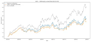
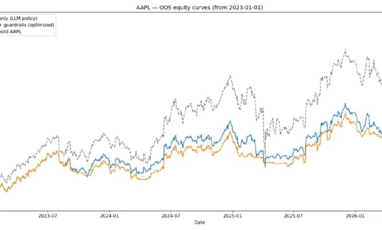
CAGR vs. Sharpe Ratio: Distinct Narratives: The strategy’s Compound Annual Growth Rate (CAGR) of 12.5% to 12.8% (depending on configuration) may appear modest when juxtaposed with the buy-and-hold benchmark’s 27.1%. However, this comparison can be somewhat misleading, as the strategies undertake fundamentally different levels of risk. The LLM-driven agents operate with annualized volatility of 14.1% and 13.9%, respectively, significantly lower than AAPL’s historical volatility of 25%. When assessed on a risk-adjusted basis, as measured by the Sharpe ratio, the performance gap narrows considerably.

Guardrails: A Trade-off Between Return and Drawdown Reduction: The integration of guardrails results in a slight reduction in CAGR, a direct consequence of the increased caution they impose. However, this comes with a significant benefit: maximum drawdown shrinks from -33% to -18%. During periods of market stress, the guardrails demonstrably prevented more substantial losses. The agent-with-guardrails version may be more suitable for risk-managed portfolios, while the agent-only version serves as a valuable baseline for quantifying the guardrails’ protective impact.

The Honest Takeaway: With the current set of state features and LLM prompt, the strategy does not consistently outperform the buy-and-hold approach in terms of absolute CAGR. The primary value proposition of the LLM in this context is not alpha generation but rather risk modulation. For investors seeking to participate in the upside potential of assets like AAPL while simultaneously mitigating the most severe drawdowns, this strategy offers a compelling framework. However, for those whose sole objective is to outperform a passive index, the development of more potent predictive features is essential, representing the most promising avenue for future research and improvement.

Reading the Equity Curves: The accompanying equity curve chart reveals three key observations. Firstly, all three curves exhibit upward trajectories throughout 2023 and 2024, confirming the strategy’s ability to participate in AAPL’s uptrend. Secondly, the "Agent + Guardrails" curve consistently tracks the "Agent-only" line during rallies but diverges downward more gradually during corrections. This divergence highlights the guardrails’ protective function: trimming exposure before losses can compound. Thirdly, the Buy & Hold strategy finishes highest due to the unusually strong uptrend and shallow corrections experienced by AAPL in 2023-2026. In more volatile or bear markets, the lower volatility and reduced drawdown characteristic of the guardrailed strategy would translate into a clearer risk-adjusted advantage, as evidenced by the Calmar ratio (0.91 for the guardrailed strategy versus 0.88 for Buy & Hold).

Step 10: Pathways to Improvement – Enhancing Strategy Performance

The developed strategy serves as a robust foundation, but its potential for enhancement is significant. The focus here is not on presenting the "perfect" strategy, but on providing actionable insights and rationale to empower users to refine their own approaches or further develop this model.

Signal Quality Enhancements:

• Multi-Horizon Momentum: Incorporating 5-day and 63-day cumulative returns alongside the current 20-day trend score provides the LLM with a more comprehensive understanding of the stock’s trend dynamics, distinguishing between early, mid, and late-stage trends.
• Earnings Blackout: Mandating a FLAT_EXP position in the two trading days surrounding AAPL’s quarterly earnings releases mitigates significant gap-risk events. This introduces no lookahead bias, as earnings dates are publicly known well in advance.
• Macro Regime Filter: Adding a binary feature indicating whether the S&P 500 is above or below its 200-day moving average provides the LLM with crucial market-wide context, particularly valuable during broad market corrections where single-stock features may lag.
• Volume Z-Score: Including today’s volume relative to its 20-day average as a state dimension can signal potential reversals (unusually low volume) or confirm momentum (unusually high volume).

Position Sizing Refinements:

• Kelly Fraction Hints: Calculating a fractional Kelly size per state from training statistics and providing it to the LLM as a sizing hint, capped at 25% of full Kelly to avoid overbetting on noisy estimates, can improve OOS Sharpe.
• Regime-Conditional Leverage Cap: During HIGH_VOL states, tightening MAX_LEVERAGE to 0.6, irrespective of volatility targeting output, prevents the reconstruction of a full position into a still-stressed market following a guardrail re-entry.
• Continuous Size Output: Prompting the LLM to output a continuous exposure value between 0 and 1, rather than discrete levels, enables finer-grained position modulation and smoother equity curves, albeit requiring more stringent output validation.

Guardrail Robustness Improvements:

• Relative Drawdown Limit: Replacing the absolute drawdown stop with one that compares strategy equity to buy-and-hold over the same window prevents premature exits during bull markets where an absolute drawdown might still represent relative outperformance.
• Noise-Filtered Volatility Stop: Requiring three consecutive days of elevated volatility before triggering the stop minimizes spurious exits caused by short-lived spikes.
• Separate Cooldowns: Implementing distinct cooldown counters for the volatility stop (e.g., 3 days) and the drawdown stop (e.g., 15 days) acknowledges that volatility spikes typically normalize faster than persistent drawdowns.
• Guardrail Optimization Frequency: Evaluating annual, semi-annual, and quarterly re-optimization cadences for guardrail thresholds can identify the optimal balance between adaptability and overfitting, potentially leading to more robust performance in slow-moving regimes.

LLM Prompting Strategies:

• Comparative Ranking Prompt: Instructing the LLM to rank all states by risk/reward and assign exposure by rank tier (e.g., top 50% get full exposure, bottom 25% get FLAT) prevents the degenerate case where the model assigns favorable ratings to all states in isolation.
• Regime Classification First: Prompting the LLM to first classify the overall market regime (BULL, CHOP, or STRESS) before setting per-state exposure ensures that all decisions are anchored to a coherent macroeconomic view and generates a loggable regime label for plotting.
• Multi-Model Comparison: Running the same prompt through alternative LLMs (e.g., GPT-4o, Claude) and comparing the resulting OOS policies can provide stronger evidence of signal quality through systematic agreement.

Evaluation Methodologies:

• Rolling Sharpe Chart: Visualizing the rolling one-month Sharpe ratio over the OOS period reveals whether the strategy’s edge is persistent or concentrated in specific lucky windows.
• Volatility-Targeted Benchmark: Including a volatility-targeted buy-and-hold strategy (which maintains constant volatility exposure) in the metrics table clarifies whether the LLM strategy genuinely adds value beyond the volatility-targeting module.
• Transaction Cost Sensitivity Sweep: Reporting results across a range of transaction costs (e.g., 0.5, 1.0, and 2.0 basis points) assesses the strategy’s resilience and the durability of its edge under varying cost assumptions.

Frequently Asked Questions:

• Q: Why employ an LLM when a simple rule could suffice?
  A: The strategy includes a direct comparison with a rule-based approach (POLICY_MODE=’rule’). If the rule outperforms the LLM, the LLM is demonstrably not adding value and can be removed. The LLM’s advantage, in this implementation, lies in its ability to provide smoother decision-making across borderline states where statistical ambiguity exists, a nuance that a rigid rule-based threshold might miss.

• Q: What is the guardrail deadlock and why is it significant?
  A: The guardrail deadlock occurs when a drawdown stop freezes the strategy’s equity at zero, preventing the drawdown from mathematically improving. This perpetuates the drawdown stop’s activation, locking the strategy in a perpetual flat state. The MAX_FLAT_DAYS re-entry counter addresses this by forcing a partial re-entry after a predetermined period.

• Q: Can this strategy be applied to other stocks?
  A: Yes, with two primary adjustments: updating the SYMBOL parameter and re-downloading relevant data. The LLM policy cache is keyed by symbol, necessitating fresh API calls for new tickers. The architecture is suitable for any liquid single stock or ETF with a substantial price history. For assets with less historical data than AAPL, reducing TRAIN_YEARS may be necessary to avoid overly sparse state statistics.

• Q: What are the API costs associated with running DeepSeek?
  A: The walk-forward loop involves approximately 40 API calls, each with a max_tokens setting of 2000. DeepSeek-chat is recognized as a cost-efficient frontier model, with the full out-of-sample run costing under $0.10 at current pricing. Once the policy cache is populated, subsequent re-runs are free of API charges.

• Q: What is the most impactful next step for performance improvement?
  A: The single most critical area for improvement lies in enhancing the quality of the state features. The current three-feature state space (trend, volatility, z-score) is relatively coarse. Utilizing a broader range of technical indicators from libraries like ta-lib holds the potential to significantly improve signal quality.

Conclusion: A Framework for LLM-Assisted Risk Management

The strategy presented herein is not a definitive alpha-generating machine, but rather a foundational framework for conceptualizing LLM-assisted risk management. The LLM earns its place not through market prediction, but by discerning subtle distinctions between market states that a simpler rule-based system might handle with a less nuanced approach.

The architecture comprises three distinct layers. Feature engineering and state bucketing transform raw price action into a format amenable to LLM analysis. The LLM prompt, deliberately framed as a risk manager rather than a forecaster, establishes a monthly exposure policy across these states. Finally, the hard guardrails, complete with their essential re-entry mechanism, ensure that no single adverse market period can permanently sideline the strategy.

The results demonstrate a strategy that effectively participates in upward market trends while significantly curtailing maximum drawdown—a valuable attribute for real-world portfolios. This is not the final iteration, however. The state features are currently coarse, the LLM prompt is version 1, and guardrail thresholds could be further optimized. Nevertheless, the underlying framework is sound, the walk-forward methodology provides an honest assessment, and every design decision is traceable.

The most effective way to learn from this implementation is to engage with it directly: run the code, identify its limitations, and rebuild it. Experiment with prompt modifications, incorporate additional momentum features, or apply the framework to different assets like SPY. The provided notebook is designed for modification, with all parameters flowing from the central settings cell.

Further Reading:

For those seeking to deepen their understanding of quantitative trading, the Learning Track: Quantitative Trading for Beginners offers foundational knowledge. To explore the practical applications of LLMs in trading, the Trading Using LLM: Concepts and Strategies track provides hands-on insights into implementing these models. For a comprehensive and advanced education, the Executive Programme in Algorithmic Trading (EPAT) covers statistical modeling, machine learning, and advanced trading strategies in Python.

References:

[Chan, 2024] E. P. Chan, "Machine Learning in Trading," YouTube, 2024. Available: https://www.youtube.com/watch?v=VzF-tvz3DAk&t=411s

Note:

The strategy concept originated from the author. The blog content was developed with the assistance of an AI large language model and subsequently curated/edited by the author.

Disclaimer: This blog is for educational and illustrative purposes only. Trading in financial markets involves substantial risk of loss. The code and concepts discussed here are not financial advice. Always exercise caution and thoroughly understand any automated trading system before deploying it in a live environment.